Fractional Brownian motion

In probability theory, a normalized fractional Brownian motion (fBm), also called a fractal Brownian motion, is a continuous-time Gaussian process B_H(t) on [0, T], which starts at zero, has expectation zero for all t in [0, T], and has the following covariance function:

$E[B_H(t) B_H (s)]=\frac{1}{2} (|t|^{2H}%2B|s|^{2H}-|t-s|^{2H}),$

where H is a real number in (0, 1), called the Hurst index or Hurst parameter associated with the fractional Brownian motion. It was introduced by Mandelbrot & van Ness (1968).

The value of H determines what kind of process the fBm is:

if H = 1/2 then the process is in fact a Brownian motion or Wiener process;
if H > 1/2 then the increments of the process are positively correlated;
if H < 1/2 then the increments of the process are negatively correlated.

The increment process, X(t) = B_H(t+1) − B_H(t), is known as fractional Gaussian noise.

1 Background and definition
2 Properties
3 Sample paths
- 3.1 Method 1 of simulation
- 3.2 Method 2 of simulation
4 See also
5 References

Background and definition

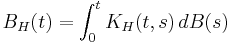
Prior to the introduction of the fractional Brownian motion, Lévy (1953) used the Riemann–Liouville fractional integral to define the process

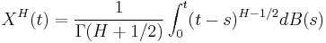
$X^H(t) = \frac{1}{\Gamma(H%2B1/2)}\int_0^t (t-s)^{H-1/2} dB(s)$

where integration is with respect to the white noise measure dB(s). This integral turns out to be ill-suited to applications of fractional Brownian motion because of its over-emphasis of the origin (Mandelbrot & van Ness 1968, p. 424).

The idea instead is to use a different fractional integral of white noise to define the process: the Weyl integral

$B_H (t) = B_H (0) %2B \frac{1}{\Gamma(H%2B1/2)}\left\{\int_{-\infty}^0\left[(t-s)^{H-1/2}-(-s)^{H-1/2}\right]\,dB(s) %2B \int_0^t (t-s)^{H-1/2}\,dB(s)\right\}$

for t > 0 (and similarly for t < 0).

Properties

Self-similarity

The process is self-similar, since in terms of probability distributions:

$B_H (at) \sim |a|^{H}B_H (t).$

Fractional Brownian motion is the only self-similar Gaussian process.

Stationary increments

It has stationary increments:

$B_H (t) - B_H (s)\; \sim \; B_H (t-s).$

Long-range dependence

For H > ½ the process exhibits long-range dependence,

$\sum_{n=1}^\infty E[B_H (1)(B_H (n%2B1)-B_H (n))] = \infty.$

Regularity

Sample-paths are almost nowhere differentiable. However, almost-all trajectories are Hölder continuous of any order strictly less than H: for each such trajectory, there exists a constant c such that

$|B_H (t)-B_H (s)| \le c |t-s|^{H-\varepsilon}$

for every ε > 0.

Dimension

With probability 1, the graph of B_H(t) has both Hausdorff dimension and box dimension of 2−H.

Integration

As for regular Brownian motion, one can define stochastic integrals with respect to fractional Brownian motion, usually called "fractional stochastic integrals". In general though, unlike integrals with respect to regular Brownian motion, fractional stochastic integrals are not Semimartingales.

Sample paths

Practical computer realisations of an fBm can be generated, although they are only a finite approximation. The sample paths chosen can be thought of as showing discrete sampled points on an fBm process. Three realisations are shown below, each with 1000 points of an fBm with Hurst parameter 0.75.


H = 0.75 realisation 1	H = 0.75 realisation 2	H = 0.75 realisation 3

Two realisations are shown below, each showing 1000 points of an fBm, the first with Hurst parameter 0.95 and the second with Hurst parameter 0.55.


H = 0.95	H = 0.55

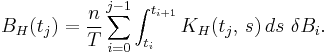
Method 1 of simulation

One can simulate sample-paths of an fBm as any Gaussian process of known covariance. Suppose we want to simulate the values of the fBM at times $t_1, \ldots, t_n$ .

Form the matrix $\Gamma=\bigl(R(t_i,\, t_j), i,j=1,\ldots,\, n\bigr)$ where $\,R(t,s)=(s^{2H}%2Bt^{2H}-|t-s|^{2H})/2$ .

Compute $\,\Sigma$ the square root matrix of $\,\Gamma$ , i.e. $\,\Sigma^2 = \Gamma$ . Loosely speaking, $\,\Sigma$ is the "standard deviation" matrix associated to the variance-covariance matrix $\,\Gamma$ .

Construct a vector $\,v$ of n numbers drawn according a standard Gaussian distribution,

If we define $\,u=\Sigma v$ then $\,u$ yields a sample path of an fBm.

In order to compute $\,\Sigma$ , we can use for instance the Cholesky decomposition method. An alternative method uses the eigenvalues of $\,\Gamma$ :

Since $\,\Gamma$ is symmetric, positive-definite matrix, it follows that all eigenvalues $\,\lambda_i$ of $\,\Gamma$ satisfy $\,\lambda_i\ge0$ , ( $i=1,\dots,n$ ).

Let $\,\Lambda$ be the diagonal matrix of the eigenvalues, i.e. $\Lambda_{ij} = \lambda_i\,\delta_{ij}$ where $\delta_{ij}$ is the Kronecker delta. We define $\Lambda^{1/2}$ as the diagonal matrix with entries $\lambda_i^ {1/2}$ , i.e. $\Lambda_{ij}^{1/2} = \lambda_i^{1/2}\,\delta_{ij}$ .

Note that this makes sense because $\lambda_i\ge0$ .

Let $\,v_i$ an eigenvector associated to the eigenvalue $\,\lambda_i$ . Define $\,P$ as the matrix whose $i$ -th column is the eigenvector $\,v_i$ .

Note that since the eigenvectors are linearly independent, the matrix $\,P$ is inversible.

It follows then that $\Sigma = P\,\Lambda^{1/2}\,P^{-1}$ because $\Gamma= P\,\Lambda\,P^{-1}$ .

Method 2 of simulation

It is also known that

$B_H (t)=\int_0^t K_H(t,s) \, dB(s)$

where B is a standard Brownian motion and

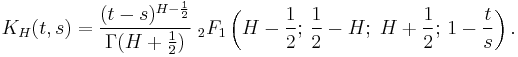
$K_H(t,s)=\frac{(t-s)^{H-\frac{1}{2}}}{\Gamma(H%2B\frac{1}{2})}\;_2F_1\left (H-\frac{1}{2};\, \frac{1}{2}-H;\; H%2B\frac{1}{2};\, 1-\frac{t}{s} \right).$

Where $_2F_1$ is the Euler hypergeometric integral.

Say we want simulate an fBm at points $0=t_0< t_1< \cdots < t_n=T$ .

Construct a vector of n numbers drawn according a standard Gaussian distribution.

Multiply it component-wise by √(T/n) to obtain the increments of a Brownian motion on [0, T]. Denote this vector by $(\delta B_1, \ldots, \delta B_n)$ .

For each $t_j$ , compute

$B_H (t_j)=\frac{n}{T}\sum_{i=0}^{j-1} \int_{t_i}^{t_{i%2B1}} K_H(t_j,\, s)\, ds \ \delta B_i.$

The integral may be efficiently computed by Gaussian quadrature. Hypergeometric functions are part of the GNU scientific library.

References

Beran, J. (1994), Statistics for Long-Memory Processes, Chapman & Hall, ISBN 0-412-04901-5 .
Lévy, P. (1953), Random functions: General theory with special references to Laplacian random functions, University of California Publications in Statistics, 1, pp. 331–390 .
Mandelbrot, B.; van Ness, J.W. (1968), "Fractional Brownian motions, fractional noises and applications", SIAM Review 10 (4): 422–437, JSTOR 2027184 .
Samorodnitsky G., Taqqu M.S. (1994), Stable Non-Gaussian Random Processes, Chapter 7: "Self-similar processes" (Chapman & Hall).